5. Running GLOFRIM
5.1. GLOFRIM workflow
By applyting the BMI functions (see :The BMI ), the following workflow is followed in GLOFRIM. The example shows coupling between a hydrologic and a hydrodynamic model, but would be identical if other or more models were coupled.
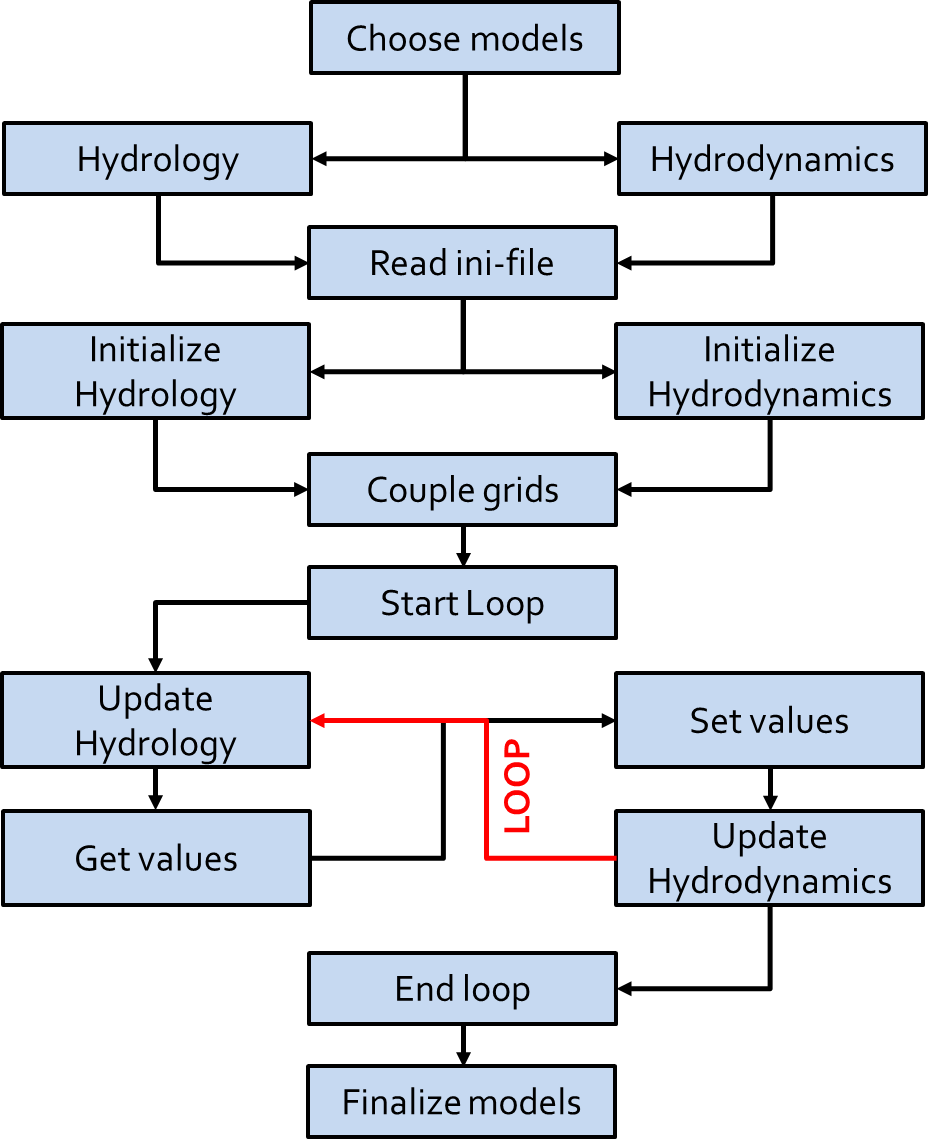
After the model are chosen and coupling settings are defined in the GLOFRIM ini-file, the ini-file is read by GLOFRIM to first initialize the model-specific configuration files and then initialize both models as a coupled entity.
Essential part of creating the coupled entity is the coupling of grids which is explained in more detail in Model coupling.
Once the coupled models are initialized, a loop is entered, starting at the start time and terminating at the end time as specified in the python executiont command (see Run GLOFRIM from command line).
During the loop, models are individually updated from the upstream end of the model cascade to the most downstream model, depending on the number of models coupled.
After a model is updated, the variables to be exchanged (as defined in GLOFRIM ini-file) are retrieved from the providing model, if necessary aligned, and inserted to the receiving model. Only then, model time of the receiving model is forward integrated until the model time of the providing model is reached.
If model end time is reached, model execution is finalized.
5.2. Run GLOFRIM from Python
GLOFRIM exists of a series of uniformed BMI wrappers for each model and a overarching BMI wrapper for running coupled models.
5.2.1. Coupled run
To run a coupled model from python use the following lines. The glofrim.ini (see example in root directory) configuration file hold the information of the individual model configuration files and exchanges between the models.
# import GLOFRIM
from glofrim import Glofrim
# initialize coupled bmi
cbmi = Glofrim()
# initialize the coupling with the glofrim.ini configuration file
cbmi.initialize_config(/path/to/glofrim.ini)
A basic model run uses the following statements:
# optional: get the model start time
bmi.get_start_time()
# initialize model
bmi.initialize_model()
# run until set endtime
bmi.update_until(bmi.get_end_time())
# finalize model
bmi.finalize()
5.2.2. Stand-alone run
To run stand alone models via the GLOFRIM BMI wrapper you can use the lines below, followed by the same statements as before.
# import the CaMa-Flood bmi wrapper
from glofrim import CMF
# intialize bmi with reference to engine (only for non-python models)
bmi = CMF(/path/to/model_engine)
bmi.initialize_config(/path/to/model_configuration_file)
5.3. Run GLOFRIM from command line
The GLOFRIM library contains a script to run combined and single models with a single line from a terminal. This script can be found in the glofirm-py/scripts folder.
GLOFRIM can be executed as follows on Linux command line:
python glofrim_runner.py run /path/to/glofrim.ini --env /path/to/glofrim.env -s startdate -e enddate
Both startdate and enddate must be in yyyy-mm-dd format.
For more info on coupled runs, check:
python glofrim_runner.py run –help
and for stand-alone runs:
python glofrim_runner.py run_single –help
5.4. The GLOFRIM configuration file
The GLOFRIM configuration (or .ini) file has four sections, the engines, models, coupling and exchanges settings, each is shortly explained here.
5.4.1. engines
The engines section contains paths to the shared libraries of each non-python model. For convenience the absolute paths in the engine and models sections may also be set in a seperate environment.env file in the GLOFRIM root folder.:
[engines]
# path to model engines; only required for the non-python models used
# these settings can also be set in environment.env
CMF = /path/to/libcama.so
DFM = /path/to/libdflowfm.so
LFP = /path/to/liblisflood.so
5.4.2. models
The models section needs the paths to all model configuraiton files. Together with the model engine, this allows GLOFRIM to know the model schematisation and to communicate with that model via BMI. Add only models which are part of the (coupled) run. The paths should be either relative to the root_dir option (if set), this ini file directory or absolute.:
[models]
# alternative root dir for relative ini-file paths, by default the directory of this ini file is used;
# this setting can also be set in environment.env
root_dir = /path/to/models

# all models which are listed here are run during update
# format: model_short_name = /path/to/configuration_file
PCR=/path/to/pcrglobwb.ini
WFL=/path/to/wflow.ini
CMF=../rel_path/to/input_flood.nam.org
LFP=/path/to/lisflood.par
DFM=rel_path/to/dflowfm.mdu
Note
Note that the user can change model options through the GLOFRIM API. For all models but WFL, a new configuration file name ending with _glofrim is written to communicate these changes with the model before model initialization. For WFL it’s possible to communicate these changes directly via BMI.
Note
CMF only listens to the configuration file if it is called input_flood.nam, therefore the original configuration file should be called different, for instance input_flood.nam.org.
5.4.3. coupling
The coupling section contains general settings for the exchanges between models. dt indicates the time step at which information should be exchanged between models. This usually should be at least one full time step of the model that runs with the largest time step. In the example we assume that a WFlow model dictates daily time steps, and that a coupled lisflood model has smaller time steps.
The section furthermore contains projections of the different model instances. GLOFRIM then reprojects the models to enable spatially correct coupling. The projections can be provided in EPSG code (e.g. “EPSG:4326” would indicate regular WGS84 lat lon projection) or as proj string, as shown in the example.:
[coupling]
# timestep for exchanges [sec]
dt=86400
WFL=+proj=longlat +ellps=WGS84 +datum=WGS84 +no_defs
LFP=+proj=utm +zone=34 +south +ellps=WGS84 +datum=WGS84 +units=m +no_defs
5.4.4. exchanges
The exchanges section contains the information about how the models communicate on run time. This part has a slightly complex syntax as it contains a lot of information. Every line indicates one exchange from the left (upstream/get) model.variable to the right (downstream/set) model.variable. This can be further extended by multipliers which can be model variables or scalar values in order to make sure the variable units match. Behind the @ the spatial location to get (upstream) and set (downstream) the model variables. Current options are @1d, @1d_us (the most upstream 1d cells or nodes) and @grid_us (the upstream cell for each grid cell). Finally, behind the location of the downstream/set model, a user may set a | sign and then specify the grid cell coordinates (in the projection of the model) in python list form, that should be coupled with the upstream grid cells of the upstream/get model. This should be done as follows:
[[x1, y1], [x2, y2], [x3, y3], ...., [xn, yn]]
GLOFRIM will then only couple these specific grid cells rather than automatically lookup which cells are coupled. This is an important feature when river networks of the upstream/get and downstream/set models are not entirely commensurate. Examples are provided below:
[exchanges]
# setup exchanges which are executed during the coupled update function.
# format: From_model.var1*var2*multiplier@index = To_model.var*multiplier@index
# the multiplier is optional; if no index is set, by default the whole 2D domain is coupled

# Example 1: PCR runoff [m] to CMF runoff [m]
# The interal CMF interpolation matrix is used to convert from the PCR grid to the CMF U-Grid.
PCR.runoff=CMF.roffin

# Example 2: PCR runoff [m] & upstream discharge [m3/s] to DFM rain [mm] (used as api for lateral inflows)
# both sides are converted to volumes per exchange timestep [m3/day]
PCR.runoff*cellArea=DFM.rain*ba*1000@1d
PCR.discharge*86400@grid_us=DFM.rain*ba*1000@1d_us

# Example 3: upstream WFL discharge (RiverRunoff) is fed into a limited set of user specified LFP grid cells at the upstream bounds of the model domain.
# The user must ensure that the selected grid cells are overlapping with the intended
# WFL major streams.
WFL.RiverRunoff*86400@grid_us=LFP.SGCQin*86400@1d_us|[[677250, 8346250], [733250, 8428750], [839750, 8398750], [688750, 8452250], [792750, 8295750]]
Note
Note that only fluxes were tested as receiving variables. While states can be used as well, their rather static nature (i.e. using m3 instead of m3/s) can lead to numerical stabilities per time step. Careful testing of the established model coupling is thus necessary!